
Caleb’s Concepts: Do blue states earn more?

February 5, 2021
Unless you’ve been living under a rock, you know that Pew Research polls show the U.S. is more divided now than ever over basic facts and politics.
According to Pew Research, 83% of voters said the winner of the 2020 election “really mattered.” Of that pool, 71% of Donald Trump’s supporters said their vote was for Trump, while 63% of President Joe Biden’s supporters said they voted for Biden. To sum this up, political lines have been drawn.
Despite having a controversial presidency, Trump’s bright spot remained the economy pre-COVID-19. Economic activity is often boring and difficult for most to understand, yet this does not stop people from forming opinions about its function.
Capitalizing on this vacuum, economic theory is determined by lawyers and politicians, who use economics for political ends.
Regardless of what your postmodern professor will tell you, there are right and wrong answers — and the truth is always in the data. Let’s explore it, shall we?
For this exploration, we examine 2018 household income from the U.S. Census, 2018 state income tax brackets from the Tax Foundation, a non-partisan organization that analyzes federal and state taxes, 2018 state legislature control from National Conference of State Legislatures and 2018 bachelor’s degree holders per state from the National Center for Education Statistics. When combined, what does the data say?
Depicted below are three charts showing the distribution of median income in states with a Democrat serving as their governor.
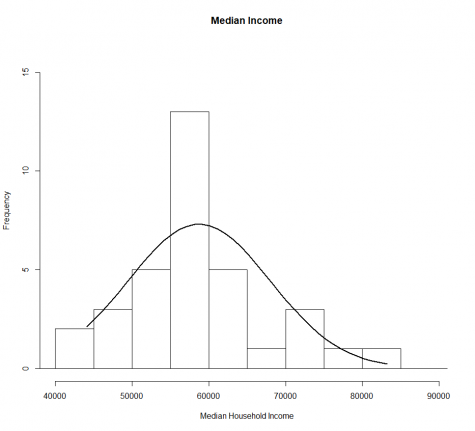
The data shows that the average state in the U.S. has a median income of $61,549.28. The Central Limit Theorem tells us that over 99% of U.S. wages are between $30,997.22 and $92,101.34.
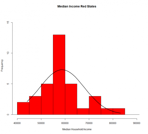
Now, let’s break up red and blue states separately.
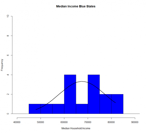
Blue states have an average household income of $67,556.44 and 99% of their wages are between $38,619.37 and $96,493.51.
On the other hand, red states have an average income of $58,722.38 and 99% of wages fall between $30,904.85 and $86,539.91.
This means that, on average, blue states have higher household incomes than red ones.
However, both the lowest and highest-earning states have Republican governors, at $44,097 and $83,242, respectively.
Now let’s examine how blue a state is. To test how red or blue a state was, we will use the proportion of the state’s legislative branch controlled by Congress. For example, blue states range between 50% and 100% with 100% representing total democrat control. A redder state ranges from 0 to 50% with 0 having no democrats. Depicted below is a scatterplot showing Democrat control and wages.
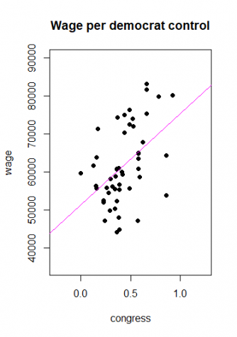
The data shows that wages will increase by $195.47 for every 1% increase in Democrats controlling education legislation.
Basically, if the whole of Congress was controlled by Democrats, this equation predicts $19,547 to states’ median incomes. Clearly, Democrats are better for the people. Let’s vote more of them into office!
Okay, Republicans, please don’t freak out. I have misled you up to this point.
I have omitted key variables that explain this phenomenon.
Depicted below is a scatterplot of the proportion of a state with at least a bachelor’s degree:
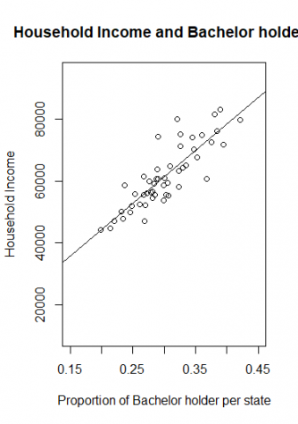
Here is the linear relationship between household income and the proportion of a state’s population that holds a bachelor’s degree. Since the data from this scatterplot fits nicely onto a line, it is clear that bachelor’s degrees are more correlated than Democrat control.
We are now ready to test the full hypothesis with more variables. Let’s combine tax policy, education, age, governor and congressional representation to see the full effect. The first model will show us the percentage increase in wages depending on the percentage increase in different variables. Model 1 is depicted below:
|
Model 1 |
|
| Intercept Coefficient | 13.67283 (p <0.01) |
| log(bachelor) | 0.78548 (p < 0.01) |
| log(Age) | -0.46806 (p < 0.05) |
| log(Top tax) | 0.0230 (p < 0.05) |
| log(Median tax) | -0.0321 (p < 0.10) |
| Governor | -0.01186 not statistically significant |
| log(Congress) | 0.09130 not statistically significant |
| R-Squared | 0.8103 |
Model 1 shows that neither a Democratic Congress nor a Democratic governor has a significant effect on the wages of a state. Bachelor’s degree holders, age and taxes affect state wages. Political control is not correlated with higher wages.
The data shows that political control does not affect wages. Since parties don’t affect wages we need to find a better model. This time we will add an interaction variable between the top tax and the median income tax. Interaction variables show how different variables interact with one another. In this case, we want to see how the top tax will interact with the median income tax. Model 2. is depicted below:
|
Model 2 |
|
| Intercept | 13.34961 (p < .01) |
| log(bachelor) | 0.82329 (p < .01) |
| log(Age) | -0.34727 (p < .05) |
| log(Top Tax)*converted | 0.10035 not statistically significant |
| log(Median Tax)*converted | -0.038 (p < .01) |
| log(interaction tax)*converted | 0.3371 (p < .01) |
| R-squared | 0.8363 |
| * The converted reference refers to the process of standardization. Because there were zero tax rates I could not convert *converted to log form. Thus, the coefficient had to be standardized by dividing the coefficient by 100 to obtain the percentage increase. | |
Model 2 is better at predicting behavior than Model 1 since it has a higher R-squared. It is important to note that the interaction term between the top tax rate and the median tax rate separate the positive effect of the top marginal tax rate. This means that taxes on the wealthiest individuals have a positive interaction with the median wage tax rate and will increase the overall wage. However, this statistical robustness may be misleading since the effect of the interaction between the top tax rate and median income tax is a low number. Its distribution is depicted below:
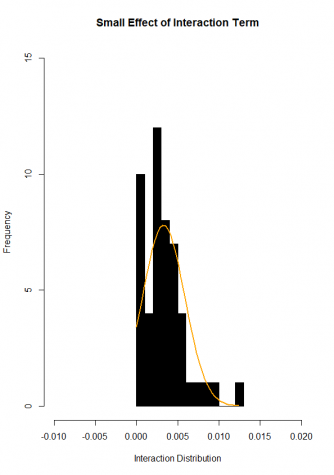
As you can see above, the data is concentrated around 0 and .015 or zero and 1.5%. This means that it would be rare for the top tax rate to increase by a magnitude to augment the real wages. For example, in a model that looks at the effect of wages, the interaction shows that a full 100% tax rate would increase wages by $2,229,574.10. However, since the average interaction is .3% the likely effect of a top tax rate that changes interaction term while holding medium tax constant would be $7,341.59. While taxes play an enormous role in increasing wages, it is important to remember other important variables. Bachelor’s degrees have the greatest statistical significance of all variables analyzed. Model 2 demonstrates that a 1% increase in a state’s population holding a bachelor’s degree will be a 0.82% increase in real wage. That may not seem like a lot; however, it results in a $1,705.42 increase in state income should the proportion of state residents holding bachelor’s degrees increase by 0.01.
In conclusion, politics gets an unfair amount of coverage on the news. Based on this analysis, this author finds no correlation between people’s wallets and whether a donkey or an elephant controls the executive or legislative branch. Rather, education, tax brackets for a state’s median income, the interaction between tax rates and age determine the median household income. However, there are some limitations, poverty rates were not factored into this model and blue states may spend more money on education programs which is correlated to success. However, there is enough evidence at the moment to show that at the end of the day, we are all humans who have hopes and dreams. Love one another.


Rudy • Nov 6, 2021 at 11:26 am
You’re article did much to obfuscate the material, and tried very hard to make Red States look halfway decent.
Here a bit more of clarification. The 19 Blue States create 81% of the National GNP. The 31 Red States create only 18% of the GNP.
For every $10 a Blue State taxpayers puts in for Federal tax, he takes out $1 in Federal services. For every $1 a red state taxpayer puts in the pot, he takes out $9 in Federal services.
The average hourly wage in Blue States is $25 and hour. The average wage in red states is $12.67 and hour.
The 15 poorest American states are red states.
The 11 states with lowest quality of living are red states.
Ben • Feb 7, 2021 at 11:21 am
Objective analysis, courageous opinions and a very compassionate conclusion from a young voice in the middle of our culture influenced by a media with a divisive agenda, of lack of leadership and distracting principles of obsessive concerns with race and gender.
Congratulations for your valiant attitude.